Most of data that I am analysing have columns with a date and time so when I create a pivot table that include those columns, excel doesn’t show correctly the information. To display correctly, I need to do some setting changes. Imagine that I have this data:

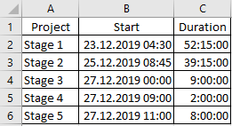
When I create the pivot table, I got this:

After doing some changes, I will get this:

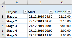
If you have the same issue, you will need to do:

• 1. Create the pivot table then put all fields in “rows”
  
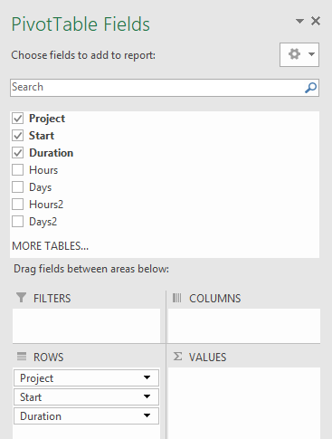
  NOTE: when I put “start” and “duration”, automatically excel will add “hours, days, hours2 and days2”, remove them from “rows”
• 2. Right click on the pivot table to select “pivottable options”
  
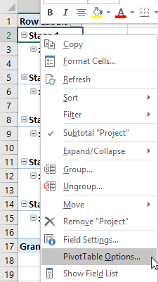
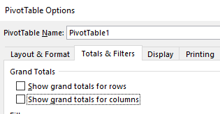
  a. In “totals & filters”, uncheck those options to not show all totals
  
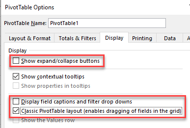
  b. In “display”, uncheck/check as shown
  
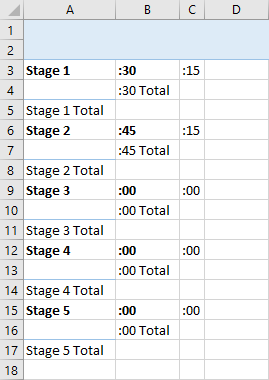
  NOTE: if all go well, I will have this:
  
• 3. Right click on the column A of the pivot table to select “field settings”
  
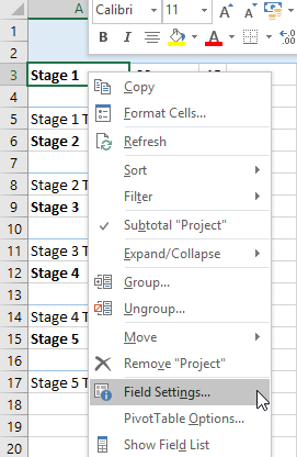
  a. In “subtotals & filter”, select “none”
  
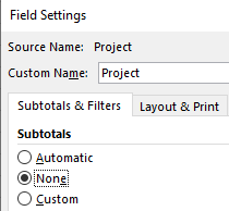
  b. Do the same thing for the 2 other columns
• 4. Right click on the column B of the pivot table to select “ungroup”
  
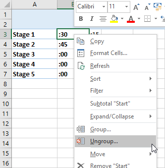
  a. Do the same thing for the column C (if need be the column A also but for this example no need)
  b. Adjust the columns to display it correctly
  NOTE: if all go well, I will have this:
  
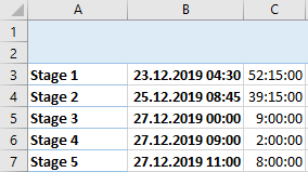
• 5. Display the title
  a. Click anywhere in the pivot table
  b. Click “analyse -> field headers”