In some of my data, I may have some numbers that are duplicated, normally I use vlookup to look for the correct data when I have only 1 unique number but when this unique number is duplicated, vlookup is not able to display what I want.

This formula is able to search and to display the data I want no matter if it is 1 unique number or if it is duplicated 2 or more times.

 

When I use the formula ?

To get the correct data when the number is duplicated.

 

How to use the formula ?

The formula in this topic is with "," so depending of the operating system of your PC, the formula should have ";" instead of ",".

For the formula to work properly, I need to do an additional action, by pressing “shift + control + enter” in order to put the formula between brackets. If not, it will show an error.

 

How is/are the formula(s) ?

=IFERROR()

=INDEX()

=SMALL()

=IF()

=MATCH()

=ROW()

=COLUMN()

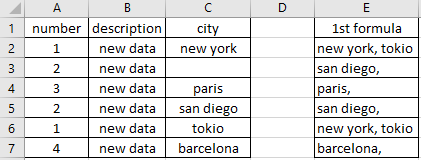
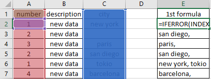
For the first formula, it is looking into 1 single column based on the number:

{=IFERROR(INDEX(C:C,SMALL(IF((A:A=A2)*(C:C<>""),MATCH(ROW(C:C),ROW(C:C)), ""),ROW($A$1)),1/(SMALL(IF((A:A=A2)*(C:C<>""),MATCH(ROW(C:C),ROW(C:C))+1/MATCH(COLUMN(C:C),COLUMN(C:C)),""),ROW($A$1))-SMALL(IF((A:A=A2)*(C:C<>""),MATCH(ROW(C:C),ROW(C:C)), ""),ROW($A$1)))),"")&", "&IFERROR(INDEX(C:C,SMALL(IF((A:A=A2)*(C:C<>""),MATCH(ROW(C:C),ROW(C:C)), ""),ROW($A$2)),1/(SMALL(IF((A:A=A2)*(C:C<>""),MATCH(ROW(C:C),ROW(C:C))+1/MATCH(COLUMN(C:C),COLUMN(C:C)),""),ROW($A$2))-SMALL(IF((A:A=A2)*(C:C<>""),MATCH(ROW(C:C),ROW(C:C)), ""),ROW($A$2)))),"")}

Pressing “shift + control + enter” to put it between brackets so I will get the result and not an empty cell.

NOTE: in this example, the number is just duplicating twice, if the number was duplicated for instance 3 times instead of 2, at the end of this formula:

1. Put:

&", "&IFERROR(INDEX(C:C,SMALL(IF((A:A=A2)*(C:C<>""),MATCH(ROW(C:C),ROW(C:C)), ""),ROW($A$2)),1/(SMALL(IF((A:A=A2)*(C:C<>""),MATCH(ROW(C:C),ROW(C:C))+1/MATCH(COLUMN(C:C),COLUMN(C:C)),""),ROW($A$2))-SMALL(IF((A:A=A2)*(C:C<>""),MATCH(ROW(C:C),ROW(C:C)), ""),ROW($A$2)))),"")

2. Change the ROW reference from 2 to 3 so ROW($A$2) to ROW($A$3)

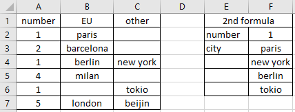
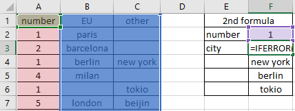
For the second formula, it is looking into the whole table based on 1 single number:

{=IFERROR(INDEX(B:C, SMALL(IF((A:A=$F$2)*(B:C<>""), MATCH(ROW(B:C), ROW(B:C)), ""), ROW(A1)), 1/(SMALL(IF((A:A=$F$2)*(B:C<>""), MATCH(ROW(B:C), ROW(B:C))+1/MATCH(COLUMN(B:C), COLUMN(B:C)), ""), ROW(A1))-SMALL(IF((A:A=$F$2)*(B:C<>""), MATCH(ROW(B:C), ROW(B:C)), ""), ROW(A1)))), "")}