vlookup and hlookup are formulas that allow to search a data in another sheet. Both work the same, the main difference is:

• For vlookup is a vertical search
• For hlookup is a horizontal search

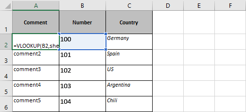
Formula 1

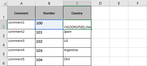
Formula 2

 

When I use the formula ?

When I need to display data of another or multiple different sheets into 1 single main resume sheet.

 

How to use the formula ?

The formula in this topic is with "," so depending of the operating system of your PC, the formula should have ";" instead of ",".

For the formula to work, you need to have at least 1 same column for all sheets. For instance, you have 3 sheets:

• Sheet1, this is the main sheet with 3 columns: comment, number, country
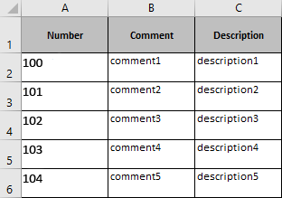
• Sheet2, the sheet with 3 columns but it is in this sheet that you will find the data for “comment”
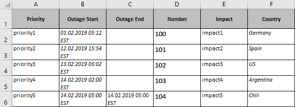
• Sheet3, the sheet with 6 columns but it is in this sheet that you will find the data for “country”

For the sheet1 to display the “country” and “comment” data, you need to have in the sheet2 and in the sheet3 the column “number”. It doesn’t matter if “number” is in column A, B, C or Z, etc.

Sheet2

Sheet3

 

How is/are the formula(s) ?

=VLOOKUP()

=HLOOKUP()

Putting the formula in sheet1:

Formula 1 (if there is a space in the name of the sheet, use the 2nd one):

=VLOOKUP(B2,sheet2!A:C,2,0)

=VLOOKUP(B2,'comment data'!A:C,2,0)

Formula 2 (if there is a space in the name of the sheet, use the 2nd one):

=VLOOKUP(B2,sheet3!D:F,3,0)

=VLOOKUP(B2,'country data'!D:F,3,0)

I will take my previous example to explain:

• Sheet1, this is the main sheet with 3 columns:
  • In the column A, in the cell A2, put the formula 1
  • In the column C, in the cell C2, put the formula 2
• =VLOOKUP(B2,sheet2!A:C,2,0)
  • B2 is the cell of the column “number” of the sheet1
  • sheet2!A:C,2
    • A is the column “number” in the sheet2 in column A
    • 2 is the numeric number counting from the column A in the sheet2
  • The formula is taking as main reference the number showing in the cell B2 and it will search in the sheet2 in the column A, if match, it will display the comment in the column B
• =VLOOKUP(B2,sheet3!D:F,3,0)
  • B2 is the cell of the column “number” of the sheet1
  • sheet3!D:F,3
    • D is the column “number” in the sheet3 in column D
    • 3 is the numeric number counting from the column D in the sheet3
  • The formula is taking as main reference the number showing in the cell B2 and it will search in the sheet3 in the column D, if match, it will display the countryin the column F

As you can see, for all sheets, we have the column “number” as the main reference for vlookup to search, it doesn’t matter that “number” is in column A or in column Z. Depending on where is located the column “number”, the formula is different:

• sheet2!A:C,2
• sheet3!D:F,3

The most important is that the first letter is where is located the column “number”. In this example:

• for sheet2, the column “number” is in column A
• for sheet3, the column “number is in column D

The second letter, C for sheet2 and F for sheet3, is doesn’t matter meanwhile the column is inside:

• for sheet2, the column “comment” is in column B so inside A:C
• for sheet3, the column “country” is in column F so inside D:F

And to end my explanation, 2 for sheet2 and 3 for sheet3, is the numeric number:

• for sheet2, counting from A to B is 2
• for sheet3, counting from D to F is 3