Last time I explained how to update automatically a trend chart using name manager in an excel report so now, I will do for a pie chart because it is quite similar but different.

It is very useful if you want to save time because if you don’t do that, each time you put the new data for the new month, you will have to update the chart after so making the chart to be updated automatically, it is a quite nice.

To explain better, I will use those data:

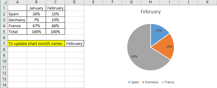
So this is how I do it:

1. Click on “formulas -> name manager”

2. Click on “new” to get this box:

3. Put a name in the “name” field (for instance “month”) and put this formula in “refers to” field:

• =OFFSET(Sheet1!$A$2,,COUNT(Sheet1!$2:$2),3,1)
• Explanation
• Sheet1!$A$2: sheet1 is the sheet name and A2 is the cell where is my data
• Sheet1!$2:$2),3,1: $2:$2 telling to take data from row 2, 3 is how many rows and 1 is how many columns
• NOTE: you can check if the formula is taking the correct data by clicking on the “refers to” field, it will highlight the area

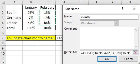
4. Close the “name manager” and select your chart then click on “design -> select data”

5. Select the month and click on “edit”

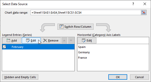
6. In “series values” field, put:

• =Sheet1!month
• NOTE: month is the name that you put in the “name manager”

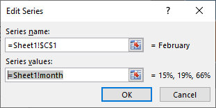
7. Click “OK” and “OK” again. Take note that if you click again in “edit”, the name will be changed from the sheet name to the excel name.

8. Now, select 1 cell and put this formula:

• =OFFSET(Sheet1!$B$1,,COUNTA(Sheet1!1:1)-1,1,1)
• In this example, I put it in the cell D7 where I have the line “to update chart month name”
• Explanation
• Sheet1!$B$1: $B$1 is referencing to the first cell I put the month, in this case “Jan”
• Sheet1!1:1)-1,1,1: it is referencing to the row where I have the month

9. Select the title of your chart and in the formula bar, put:

• =Sheet1!$D$7

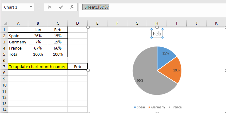
10. Now if I put the new data for the month of March, the chart will be update automatically including its name.

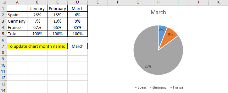
If you want to customize the title of your chart, for instance, instead to put only “march”, you want to put “SLA results for March”. In this case, read my topic Mix text and formula into a cell with a formula in an excel report.