Power BI: convert decimal to unique number for filter
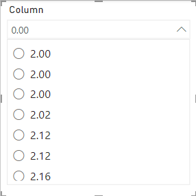
When I work with date and/or time, I can’t use decimal numbers as a vertical list, tile or dropdown slicer because usually there will be duplicate. For instance (left picture):
| single selection dropdown filter | between filter |
 |
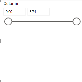 |
Of course, I can use the between filter (right picture) but based on the type of report, sometimes, I prefer to use the others. In fact, there is no issue at all using it like that but seeing multiple times same values, it is quite confusing. In my example, to select the value 2.00, it appears 3 times and I need it only 1.
Converting the column as whole number it is not a solution because it will round up or down the number. For instance, values between 2.5 and 3.5 will be 3 but if I select 3 in my slicer, I don’t want to show in my table or to calculate in my visual card everything above 3. At the end, in my mind, selecting 3 means “3 and below” and not “3 and above”. Neither using functions like ROUND, DATEDIFF, etc. will resolve it.
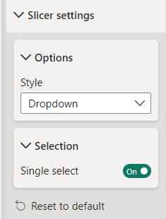
The solution I found it is to use the TRUNC function. It will extract the digits before the dot, for instance 241.56 will be 241. Here is my logic, as you can see in the picture above on the left, my filter is a dropdown one with a single selection (left picture). I need to convert it into single unique value like that (right picture):
 |
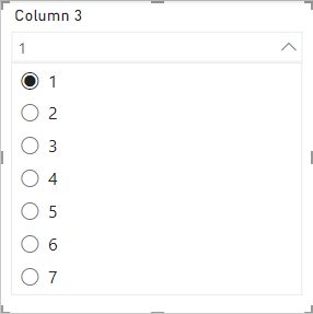 |
So when I select a number, I want to show everything equal and below meaning “2 and below” and nothing above it meaning 2.01, 2.02, etc. For that, I need to tell Power BI:
- 1. Every integer number should stay as it is. For instance, 1 = 1, 7 = 7, etc.
- 2. Every value above the integer but below the upper one should be considered as integer number. For instance 1.01 = 2, 1.47 = 2, etc.
So the result will be:
- 0.00 = 0
- 0.01 -> 0.99 = 1
- 1.00 = 1
- 1.01 -> 1.99 = 2
- 2.00 = 2
- Etc.
This is my formula:
IF('table'[argument]=TRUNC('table'[argument]),'table'[argument],((TRUNC('table'[argument])+1)-'table'[argument])+'table'[argument])

NOTE: replace table and argument by yours. In the picture above, I didn’t put the “table” because the new column is in the same table.
Let’s take a look with an example based on my scenario. This is my table:
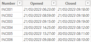
I will create a new column to know the number of closing days:
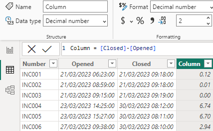
I will create another one with the same formula but formatted as whole number so we can compare:
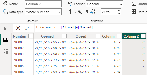
Remember I told you that putting it in whole number, it will round up or down:
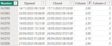
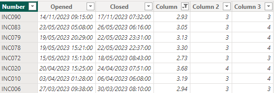
So selecting 3, I will have a range from 2.73 until 3.30 (normally it should be 2.5 until 3.5 but for my data, I don’t have those values). This is not what I want, I want by selecting 3, only the range from 2.73 until 3.00. I will create another column with my formula:
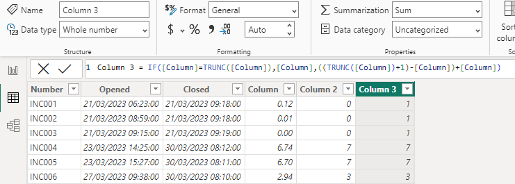
Now, we can see that numbers above 3.00, it is 4:
Interesting Topics
-

Be successfully certified ITIL 4 Managing Professional
Study, study and study, I couldn’t be successfully certified without studying it, if you are interested...
-

Be successfully certified ITIL 4 Strategic Leader
With my ITIL 4 Managing Professional certification (ITIL MP) in the pocket, it was time to go for the...
-

Hide visual and change background color based on selection
Some small tricks to customize the background colour of a text box...
-

Stacked and clustered column chart or double stacked column chart
In excel, I use a lot the combination of clustered and stacked chart...


